1 - MATERIALS

1 - 1 - Equipment

1. Computer running with Linux operating system with a minimum setup, see equipment setup.
2. DNA sequencing data, such as BLESS, or ChIP-Seq
3. Newest version of iSeq, at least core procedure, hygestat_BLESS, that can be downloaded here (download hygestat_BLESS) and all third party software as described in equipment setup section.

1 - 2 - Equipment setup

1. Hardware requirement and computer configuration:
   iSeq is a software pipeline, written mainly in C++, with some additional python, perl and shell scripts. The latest version of C++(gcc) compiler should be installed (generally comes with linux operating system, just needs to be updated), C++ libraries called boost ( download boost) and gsl ( download gsl ) have to be installed as well.
   hygestat_bless uses bowtie or bowtie2 to align the reads to the reference genome (bowtie is used as default). For information about how to install bowtie and bowtie build index, go to bowtie website (download bowtie ).
   hygestat_bless optionally uses samstat and/or fastqc (download samstat, download fastqc) to preprocess and check the quality of the data before analysis.
   A computer (64-bit), running in linux with a minimum of 2 GB of RAM, 100 GB of free space in hard drive (HD) is required to complete this tutorial.
2. Input data:
   hygestat_bless currently accepts data in fastq or fasta format from any NGS pipeline (Illumina, Roche 454 etc).
   Data can be genomic (here we consider genomic all data without a barcode) or BLESS (data with specific sequencing barcode, that can be user-defined).
   In this tutorial, we will use actual BLESS barcodes, but the procedure can be easily adapted to any type of barcoded data. Data used in this tutorial can be obtained from NCBI Sequence Read Archive (accession number SRP018506) or from our website breakome.
   Once all data and requirements have been successfully setted up, no action is needed until the end of the process with the output file written in output.txt.
3. Output data:
   containing 8 columns. These columns are, starting from the first: chromosome number, window start position, window end position, number of reads in sample of interest (treated sample) for the current window, number of reads in control (untreated sample) for the current window, p-value (calculated using hypergeometric test), q-value1 (p-value corrected for multiple hypothesis testing using Benjamini-Hochberg correction) and q-value2 (p-value corrected for multiple hypothesis testing using Bonferroni correction). An example of output file file is shown in the Table 1 bellow.

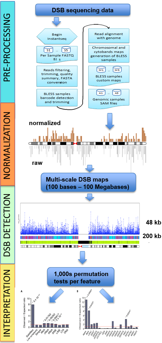
2 - PROCEDURE

2 - 1 - Overview

1. Reading input data
2. Reading input data and extracting sequence reads (in case of fastq data input).
3. Pre-processing: Data trimming (optional) and barcode removal (if barcode used).
4. Aligning to the reference genome using bowtie (download bowtie if not yet installed).
5. Loading the pre-computed mappability map for the reference genome.
6. Reading bowtie output (using provided hit.sh shell script) to produce the mapped positions for each chromosome and for each strand, saved in the directory called input_XX_barcode where XX stands for close or no barcode depending on point 3.
7. Dividing genome into intervals of user-determined length in mappable reads (the intervals that, due to low mappability, would be more than 10 times longer than the user-provided target length are skipped and the procedure is started anew)
8. Finding intervals (defined as in point 6) enriched in reads in the treated sample, using hypergeometric test (p-value is calculated separately for each window).
9. alculating Benjamini-Hochberg or Bonferroni correction to correct p-values for multiple hypothesis testing (user can choose; Bonferroni correction is more rigorous than the Benjamini-Hochberg method and recommended for very deeply sequenced data sets, such as our recent yeast data (Biernacka et al. (2017), in preparation; Zhu et al., (2017A), in preparation); Zhu et al., (2017B), in preparation);.
10. Creating an output table (eight column table (column explanation in the Table (add link) below) containing the results for each interval considered. For DSB sequencing data, the p-value indicates whether the given region is fragile (statistically significantly enriched in DNA double-stranded breaks).
11. Annotating the results: hygestat_annotation automatically finds annotations enriched in significant regions found by hygestat_BLESS, using annotations from UCSC and NCBI, or user-provided.
12. Identifying genes with significantly higher than expected numbers of reads in the treated sample (for BLESS, genes most prone to breaks) by computing the hypergeometric test for every gene (hygestat_genes software).
13. Estimating probability for user-defined regions (in bed format) having significant enrichment of reads in the treated sample (hygestat_genes software).
14. Analyzing locations of significantly fragile intervals with respect to transcription start and end sites (find_gene software).
15. 14- Visualizing data on the chromosomes using the custom Matlab procedure. The pipeline software for visualization is available at the download section of this page, follow the steps in the README file to create the plots.

2 - 2- hygestat_BLESS critical steps

1. Reading raw data and sequence read extraction.
   After successfully installing or compiling hygestat_BLESS (breakome), there are two possibilities to input the data: via command line or by using the config file, downloadable frombreakome.
   For more information about how to input the data and options of the software, please refer to our website (breakome)) and follow the instructions provided.
   In case of fastq data, the process_fastq function allows extraction of reads from fastq and produces the input.csv file containing information about the quality of the data. Troubleshooting: see troubleshooting section below.
2. Pre-processing: data trimming and barcode removal.
   In the case of barcoded data, the shell script hit.sh allows removal of the barcode before any mapping to the reference genome. The script assumes that barcodes are located only at the beginning of reads and will search for reads that start with the user-provided barcode.
3. Aligning to the reference genome.
   Reads are aligned to the reference genome using the third party software (bowtie). For more information about read alignment using bowtie, refer to the bowtie webpage (bowtie ).
4. Loading the pre-computed mappability map for the reference genome.
   To take into account genome mappability during analysis, the iSeq software uses the pre-computed genome mappability files, that are available from our website for human, mouse and yeast, or can be computed for other organisms using our mappability software package, also available from our website (click here).
5. Reading bowtie output
   The provided shell script hit.sh is used to read  bowtie output and extract read positions mapped to the reference genome.
6. Dividing genome into intervals of constant length in mappable nucleotides (user determined length).
   To reduce data complexity for further analysis, especially for annotating with known genomic features, we divide the genome into windows of equal length in mappable nucleotides, with window size defined by the user. If the actual size of the resulting window is 10-fold or bigger than user-defined (that is if the mappability is less than 10%), such window is skipped and the process is repeated from the beginning. We recommend analyzing data at the minimum of several different resolutions for spotting trends and overall more accurate results.
7. Finding enriched intervals
   The hypergeometric statistical test is used here to evaluate the probability for a given interval of being significantly enriched in treatment sample reads (i.e. being “fragile”, in case of DSB sequencing data).
8. Multiple hypothesis testing corrections
   Currently, two corrections for multiple hypothesis testing are supported: Benjamini-Hochberg correction (q-value #1) and Bonferroni correction (q-value #2). Bonferroni correction is more rigorous than Benjamini-Hochberg and is recommended for deeply sequenced samples, for example all the yeast samples. In our experience, for human and mouse samples Benjamini-Hochberg correction still gives better results, although it may change with increased depth of sequencing. Negative controls are very helpful in estimating the false positive ratio.
9. Interpretation of the hygestat_BLESS output table
   Table 1 below shows an example of a hygestat_BLESS output (named output.txt (default) or provided_name.txt). The output table consists of eight columns, with the following content:
   • Column 1: Chromosome number (chrXX).
   • Column 2: Chromosomal coordinate of window start.
   • Column 3: Chromosomal coordinate of window end (note that depending on mappability, the size of the window in nucleotides can be up to 10 times greater than the chosen window size).
   • Column 4: Number of reads from the treated sample mapped in the given window.
   • Column 5: Number of reads from the control sample mapped in the given window (note that these are raw, not normalized values, so a higher number of reads does not necessarily mean enrichment; use q-values to identify regions statistically enriched in treated sample reads, i.e. "fragile" for DSB sequencing data)
   • Column 6: The p-value for the given window is computed using the hypergeometric test. Here, the population size is defined as the sum of the total number of reads in a given chromosome for treated and non-treated samples; the sample size as the number total of reads in the given window for treated and non-treated samples; the success in population as the number of reads in the given chromosome for the treated sample; the sample size is the sum of the number of reads in the given window for treated and non-treated samples; the success in the sample is defined as the number of reads in a given window for the treated sample.
   • Column 7: p-value after Benjamini-Hochberg correction (Q-value #1). Use for samples from organisms with relatively large genomes (e.g. human, mouse).
   • Column 8: p-value after Bonferroni correction (Q-value #2). Use for samples from organisms with relatively small genomes (e.g. yeast).
   
   

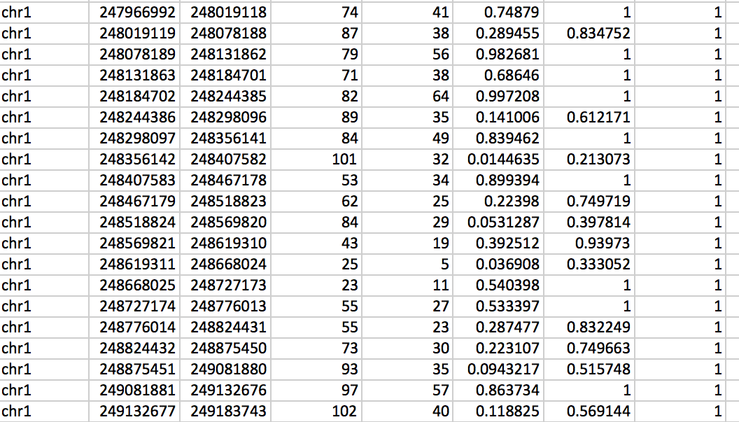
   Table 1: Example of hygestat_BLESS output template

10. Annotating the results
    Hygestat_annotation annotates enriched regions found by hygestat_BLESS using genome annotation data. Program input consists of the following files:
    1. ygestat_BLESS output (or any data file in compatible format,containing some genomic features binned into equal size (or equal size in mappable nucleotides) genomic windows),
    2. annotation file in BED or bedGraph format, containing any discrete or continuous genomic annotations, respectively,
    3. (optional) genome mappability data, imported to bitarray format.
    Hygestat_annotation calculates the overlap between significantly enriched windows, found by hygestat_BLESS, and given genomic regions (in the case of discrete annotation data) or the average feature level in significant hygestat windows (in the case of continuous annotation data). In both cases, the result is compared to the expected value for randomly selected windows of the same type and p-values for enrichment and depletion are calculated. When the mappability data are provided, the analysis is performed only in the mappable genome regions, which is recommended for the sequencing data to increase accuracy.
    Requirements: hygestat_annotation is fully written in Python. It requires Python 2.7 with package bitarray 0.8.1 installed (see bitarray for bitarray installation options).
    Usage: hygestat_annotation.py [options]

    Options

    Click here to expand/hide hygestat_annotation options

    Option	Extended option	Argument / Usage	Description	Default argument
    -h	---help		show the help message and exit
    -F	--feature-file	FFILE / --feature-file=FFILE	path to the annotation data file	[no default]
    -B	--bless-file	BFILE / --bless-file=BFILE	path to the bless data file	[no default]
    -b	--bless-name	BNAME / --bless-name=BNAME	BLESS experiment name for output data	[default: path to the bless data file]
    -f	--feature-name	FNAME / --feature-name=FNAME	annotation name for output data	[default: path to the annotation data file]
    -g	--bedgraph		produces annotation data in bedGraph format	[default: BED format]
    -O	--output-file	OUTFILE / --output-file=OUTFILE	path to the output file	[no default]
    -a	--append-output		appends output to existing file	[default: create a new file]
    -p	--pvalue-thresholds	PVTHRS / --pvalue-thresholds=PVTHRS	comma separated list of p-value thresholds for BLESS data	[default: p-value threshold is 0.05]
    -c	--pvalue-column	PVCOL / --pvalue-column=PVCOL	p-value column in bless data file	[default: 7]
    -M	--mappability-dir	MAPDIR / --mappability-dir=MAPDIR	path to the mappability data directory	[default:no mappability]
    -n	--n-tests	NTEST / --n-tests=NTEST	number of permutation tests	[default: 1000 ]

    Definitions:
    
    • FFILE: annotation data in BED or bedGraph format to be compared with BLESS data. All but the first three (BED) or four (bedGraph) fields in each line are ignored.
    • BFILE: BLESS data output from hygestat_BLESS.
    • FNAME and BNAME: input data names used in the output file (see OUTPUT FORMAT below).
    • OUTFILE: output is written as a tab-separated text file (see OUTPUT FORMAT below).
    • PVTHRS: significance level thresholds for BLESS data.
    • PVCOL: column determining p-value type for BLESS data; possible values are:
      • p-value from the hypergeometric test,
      • Benjamini-Hochberg corrected hypergeometric p-value (default),
      • Bonferroni corrected hypergeometric p-value.
    • MAPDIR: directory with the mappability data imported to binary format (see MAPPABILITY below);
    • NTEST: the number of permutations in the enrichment/depletion estimation; resulting p-value resolution equals 1/NTEST.
    Output format:
    Each row in the output file contains the following fields:
    
    1. feature - FNAME argument
    2. treatment - BNAME argument
    3. pv_threshold - BLESS p-value threshold, a component of PVTHRS argument
    4. level_all - the fraction of nucleotides overlapping with the selected feature in the genome
    5. level_fragile - the fraction of nucleotides overlapping with the selected feature within hygestat_BLESS-significant windows (or within window p-value <= pv_threshold if non-default of PVTHRS is selected)
    6. level_proportion - level_proportion - enrichment of the selected feature in hygestat_BLESS significant ("fragile") intervals (level_fragile/level_all ratio)
    7. pval_enrichment - p-value for the enrichment (level_proportion)
    8. pval_depletion - p-value for the depletion (level_proportion) .
    Mappability:
    When option -M is specified, all statistics are calculated considering only mappable nucleotides. Pre-computed mappability maps for several organisms are available in text format from our website (add link).
    In order to accelerate data loading, hygestat_annotation uses more compact binary format. Script import_mappability converts the mappability data from text to binary format.
    Usage: import_mappability.py INPUT_DIRECTORY OUTPUT_DIRECTORY
    Definition:
    INPUT_DIRECTORY : path to the directory with mappability data in hygestat_BLESS format
    OUTPUT_DIRECTORY : path to the directory for mappability data in hygestat_annotation format; if the directory does not exists, it will be created.
    
11. Analyzing enrichments in genes (hygestat_genes)
    hygestat_genes works as hygestat_BLESS (described above), but instead of using same size mappable windows for binning the data, it will assign reads to genes. To run hygestat_genes:
    1. Download the zipped package from our website. After unzipping the package ($unzip Hygestat_genes) type $cd Hygestat_genes to change directory and then $make to compile the program and obtain the executable file (hygestat_genes).
    2. Perform the command $./hygestat_genes treated_xx_barcode/ untreated_xx_barcode/ mappability_directory/ gene_code_annotation.gft, which executes the program.
    Notes: treated_xx_barcode and untreated_xx_barcode denote treated and untreated sample directories, as for hygestat_BLESS.
    Mappability_directory is the directory containing the pre-computed mappable regions across the genome. Such mappability maps are available for several organisms (human, mouse, yeast) from our webpage; we also provide the scripts to compute such maps for other organisms. Gene annotation files used by hygestat_genes can be downloaded from our website or from databases (e.g. gene_code_annotation.gtf can be obtained from UCSC Genome Browser website).
    Output format: The output file for hygestat_gene contains ten columns:
    1. Chromosome number
    2. Gene name
    3. Gene start position
    4. Gene end position
    5. Gene size
    6. Mappable length
    7. Number of reads in treatment (treated sample) for the given gene.
    8. Number of reads in control (untreated sample) for the given gene.
    9. P-value for the given gene being enriched in breaks (or other measured characteristic) (hypergeometric test).
    10. Q-value, i.e. p-value corrected for multiple hypothesis testing (Benjamini-Hochberg correction).
    
    The content of the columns is described in more detail in Table 2 below.
    
    

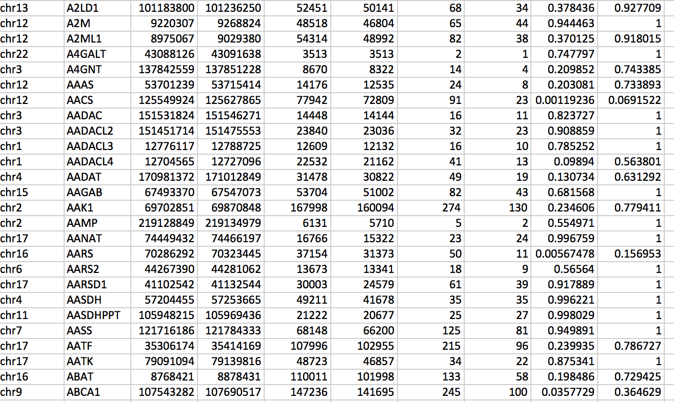
    Table 2: Example of an output file produced by hygestat_genes.

12. Analyzing enrichments in user-provided intervals (hygestat_bed)
    Hygestat_bed uses custom regions, provided by the user, to evaluate enrichment of DNA breaks (or other measured feature), in these regions. To use, download the zipped package called Hygestat_bed.zip from our website. After unzipping the package ($unzip Hygestat_bed.zip), type $cd Hygestat_bed to change the directory and $make to compile the program and obtain the executable file (hygestat_bed).
    Use the following command to execute the program: $./hygestat_bed treated_xx_barcode untreated_xx_barcode size_window bed_regions
    Notes:treated_xx_barcode and untreated_xx_barcode are treated and untreated samples (as in hygestat_BLESS).
    A bed_file is a text file with three or more tab separated columns that contain the chromosome numbers and genomic addresses (begin and end coordinates) of some genomic regions of interest. Fourth and further columns of a bed file are ignored by hygestat_bed.
    Additionally, an option specifying minimum window size to be accepted among those provided in the bed file can be used (default is 1, that all windows in the user-provided bed file are analyzed): $./hygestat_bed treated_xx_barcode untreated_xx_barcode size_window bed_regions.
    The output of hygestat_bed (see also Table 3) contains the following eleven columns:
    
    1. Chromosome number (chrXX)
    2. 2. Window beginning address
    3. 3. Window end address
    4. Window size
    5. 5. Number of treatment reads in the given window
    6. 6. Number of control reads in the given window
    7. 7. P-value for the given window to be enriched (obtained from the hypergeometric test)
    8. 8. Q-value1 (calculated using Benjamini Hochberg multiple hypothesis testing correction)
    9. 9. Q-value2 (calculated using Bonferroni multiple testing correction. Bonferroni method yields more conservative q-values than the Benjamini-Hochberg method and is thus recommended for deeply sequenced samples, where sensitivity of the detection is not a concern)
    10. -Log of p-value
    11. -Log of q-value1
    12. -Log of q-value2
    
    

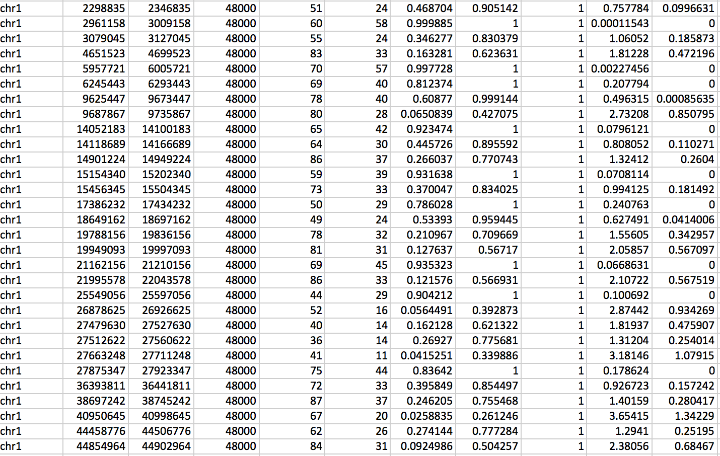
    Table 3: Example of hygestat_bed output table

13. Analyzing locations of significant regions with respect to transcription start and end sites (find_gene)
    This function uses the hygestat_BLESS (or hygestat_bed) output to find the nearest genes for each region.
    The user can determine in which distance from transcription start sites or ends to search for enriched intervals found by other hygestat_programs.
    The software also returns the orientation of the found fragment vs. gene. For example, whether an enriched region was found upstream/in the gene promoter (user can define distance cut-off), within a gene body, or downstream. This functionality can be used for example to analyzing if DSBs are enriched in promoters of differentially expressed genes, as we did in (cite).
    It can be obtained from our website (breakome/software) and it works as follow: Download the zip package from our website and after unzipping it, type $cd Find_gene to change the directory and $make to get the executable file.
    To execute the program, use the following command: $./find_gene hygestat_window_output.txt gene_code_annotation.gtf distance_parameter p-value_threshold.
    The output file (Table 4) can be found in output.txt and is interpreted as follow:
    1. Chromosome name (chrXX)
    2. Gene name
    3. Gene start position
    4. Gene end position
    5. Strand
    6. Window start position
    7. Window end position
    8. Distance from gene
    9. Gene position
    10. P-value
    11. Distance parameter
    
    

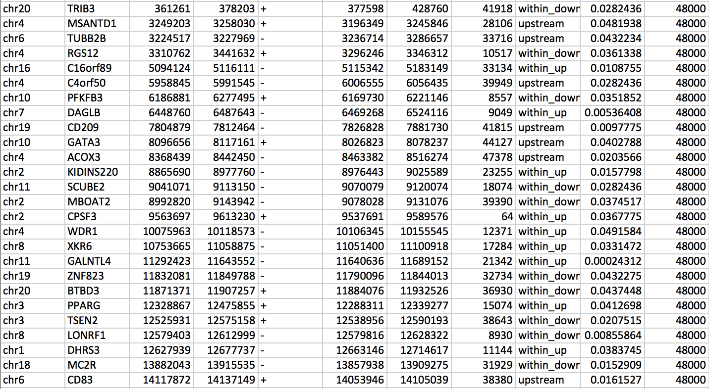
    Table 4: Eleven columns table results showing an overview of the find genes program output

14. Visualizing the data on the chromosomes using custom Matlab code
    The pipeline software for visualization is available on our website to be downloaded (breakome). Follow the steps on the readme file to obtain the plots.
15. TROUBLESHOOTING
    
16. TIMING
    The computational time for the whole analysis entirely depends on the data set and size, however:
    1. Steps 1 – 3 read the data, extracting reads, and removing barcodes takes less then 10min
    2. Step 4, aligning fragment reads to the reference genome takes less than 35min
    3. Step 5, Reading bowtie output and extracting mapped position take less than 3min
    4. Step 6, Reading of pre-computed mappable regions and finding reads overlapped with those mappable regions. This process takes less than 5min
    5. Steps 7-10, evaluate p-values for each region and writing the output file, this process takes less than 5min
    6. Step 11, finding the annotation of the data with the well-known data from genome browser (NCBI) takes about 30 min depending of the precision of the results
    7. Step 12, Running hygestat genes function to find gene prone fragility takes no longer than 10min
    8. Step 13, Running hygestat bed regions to evaluate the probability of given regions of being fragile or double strand breaks (DSBs) prone regions. This process takes less than 10 min
    9. Step 14, Finding the surrounding genes of the region of interest by running find genes function. This process takes no longer than 1h depending of the distance parameter (distance from the region of interest)

    Based on the advanced with computational tools, today’s computational timing should not be the limit for the high quality of analysis. We test the computational timing for the whole data set from Crosetto et al. during this protocol. Running the whole process in a DELL machine (characteristics) for hygestat window takes no longer than 40min. The most timing process is to align the reads to the reference genome. As others software use the pre-processing data from hygestat window (mapped data and hygestat window output), the computational time is considerably reduced and vary from 2min to 10min.

17. ANTICIPATED RESULTS
    In this section, we applied each step described above to the data from Crosetto et al. and recovered the results as described in the publication. The data can be obtained under accession number SRP018506 or from our website (breakome). Following the steps given above (procedure), we show in this section the distribution of DNA double strand breaks (DSBs) across each chromosome as described in the original paper (Crosetto et al.). Figure 3 bellow presents the regions prone DSBs for each chromosome.
    
    

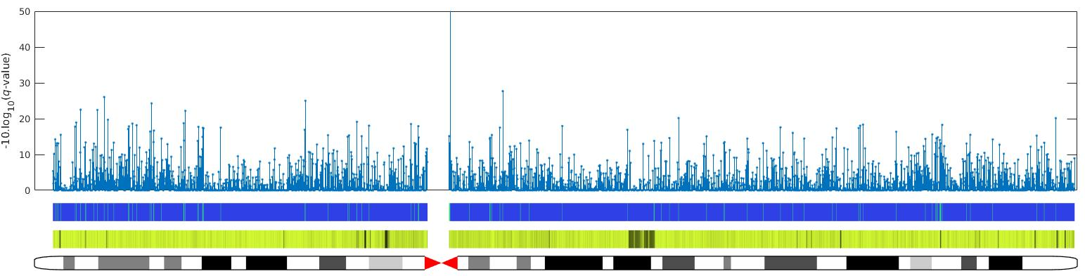
    Fig 3: An example of chromosome X (human genome) using data from Nature Method (Crosetto et all.) to show the distribution of DSBs across the chromosome. The top panel represents the -10log(q-val) for each region on the chromosome with 48k window size. In the second panel from the top, the green bars represent the regions prone DSBs. The third panel represents 48kbp mappability region with black bars as non-mappable regions.